How AI Predicts Starbucks Customer Conversions
Introduction
Every few days, the Starbucks team sends out offers to users of their mobile app. There are three main types of offers: discount, bogo (buy one get one) and informational offers. The goal of the project was to create an offer recommendation engine to suggest the right offer for the right customer. By using customer demographic attributes such as age, income and offer attributes such as duration, required to spend, the engine can predict if the customer will respond to the offer or not. With the help of the recommendation engine, the Starbucks team will be able to increase the ROI of their marketing campaigns.
Executive Summary
The data for the project was provided by the Starbucks team. There are three different datasets. The datasets contain customer attributes, transaction data and offer attributes. The project contains the following parts: preprocessing, exploratory data analysis (EDA), feature engineering and model training. During the preprocessing part, the data was cleaned and joined together. The preprocessing part was the most time-consuming part of the project. During the exploratory data analysis phase, the data was analyzed to build simple heuristic rules:
- Discount offers show the best performance
- The longer the duration time of the offer, the better the performance
- Women on average spend \$10 more than men
- Women on average have 5% higher conversion rates
- Average customer spendings increase with the age of the customer
- The conversion rate increases with the age of the customer
- Men react to discounts better than buy one get one free offers
- Customers with an income of 100k+ react better to buy one get one free offers.
The dataset was highly imbalanced. There were less successful offers. Therefore during the feature engineering part, an oversampling method was applied to rebalance the data. Due to oversampling, the accuracy score of the final algorithm was improved by 4%. In the final phase of the project, the model training part, different algorithms were tested. The tree-based algorithms outperformed all other algorithms. To get the best results, stacking was used to build the final model. The final model was able to deliver an accuracy rate of 73%.
Results
The final result shows an accuracy rate of 73%. This means that out of 100 offers, the algorithm can predict 73 of them correctly. The Starbucks team can now see with an accuracy rate of 73%, if the offer will be accepted by the customer or not, prior to sending the offer to the customer. According to the peer-reviewer of the project, the accuracy rate of 73% has surpassed the benchmark by a large amount. To come up with the final result, different algorithms were analyzed via a brute-force method. After validating the algorithms, the tree-based algorithms showed the best accuracy rate. After the brute-force step, the decision was made to choose ensembles to see if the results could be improved. The best result was delivered by the Random Forest algorithm. Random Forest showed an accuracy rate of 71%. The optimization of Random Forest through a grid search approach didn’t show any improvements. In the last step of the project, a stacked version of Random Forest was tested. After running the stacked version of Random Forest the accuracy metric increased by 2%. The final result was achieved with an accuracy rate of 73%.
Project Overview
Three files were provided by the Starbucks team.
- portfolio.json: contained information about the offer attributes
- profile.json: contained information about the customer attributes
- transcript.json: contained information about events such as offer views and previous transactions.
Data Preprocessing
The project started with the data preprocessing part. The data preprocessing part included data cleaning, aggregation of metrics and joining of data frames. The preprocessing part is needed to transform the data in to a proper format, so it can be used for later analysis and feature engineering. For example Figure 1.0 shows an already transformed portfolio.json data frame, the channel column was dropped and converted into one-hot-encoded values for channels. Also, a specific offer_name column was constructed to have a stronger naming for the exploratory data analysis part.

Figure 1.0: Modified portfolio data frame
The profile.json data frame contained 17,000 customer records with information such as age, income, membership duration and customer id. It turns out that the profile data frame contained 2,387 rows with missing values in age, gender and income columns. Figure 1.1. shows a high-level overview heatmap of missing values. Since it was not correct to impute or to fill the values with averages, the decision was made to drop the rows with missing values.

Figure 1.1: High-level overview of missing values
The last step in the data preprocessing part was about the aggregation of metrics. The last step was the most time-consuming part of the project. The metrics aggregation was undertaken by joining the data frames and calculation of time-windows for the offers. There was no direct link to an offer to the transaction. Therefore calculation of a time-windows between offer received and offer completed was undertaken. Figure 1.2 shows the combined final data frame. Note, since some offers have overlapping time windows, the amount spent can be duplicated across the offers. There is no other way to attribute the amount spent on an offer other than doing the window-based calculation.
 Figure 1.2: Combined transactions and offer attributes data frame
The final aggregated offers data frame was joined with the customer demographic data from the profile data frame.
Exploratory Data Analysis (EDA)
Figure 2.0 shows the conversion rate by offers. Based on this information, it can be seen that the discount offer to spend \$10 with a \$2 reward within 10 days has the highest conversion rate. Next is a discount offer to spend \$7 with a \$3 reward within 7 days. The least performing offer is a discount offer to spend \$20 with a \$5 reward within 10 days. Based on this information, a decision can be made that there needs to be a balance between the amount spent and the duration of the offer.
 Figure 2.0: Conversion rate by offers
As shown in Figure 2.1, the best performing offer in terms of average spend is the discount offer, to spend \$10 with a \$2 reward within 10 days. This offer seems to be the optimal offer for the majority of the customers of Starbucks. The second-best offer in terms of conversion rate was the discount offer to spend \$7 with a \$3 reward within 7 days, performed slightly better than the average.
 Figure 2.1: Average spend by offers
In Figure 2.2 there is an overview of average spend by gender. The figure clearly shows that women spend more money than men. The difference is around \$10. Figure 2.3 shows that women have a 5% higher conversion rate compared to men. Note, the current dataset is imbalanced towards men, as there are almost 2,000 fewer female customers.
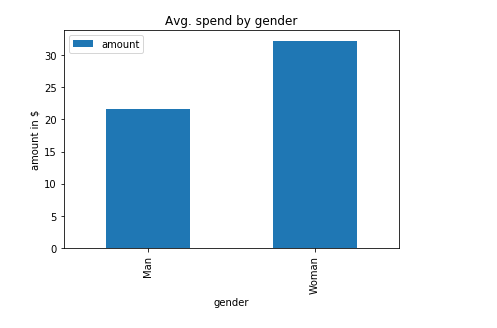
Figure 2.2: Average spend by gender
Figure 2.3 shows the difference in conversion rates by offer and gender. It can be seen that women perform well on both offers, the conversion rate is similar, while men tend to have a higher conversion rate on discount offers. The informational offer has no conversion rate because there is no way to complete that type of offer.
 Figure 2.3: Conversion rates by offer and gender
Figure 2.4 shows the conversion rate by offers and income. As shown here, people with higher incomes have a higher conversion rate on bogo offers. People with less income prefer discount offers. A general rule of thumb can be made, the higher the income the higher the conversion rate for bogo. Bogo conversion rates “correlate” to the income of a customer.
 Figure 2.4: Conversion rate by offer by income
From the exploratory data analysis part, simple heuristic rules can be derived. The derived heuristic rules can be used to construct new marketing campaigns. Since the goal of the project was to create a fully automated offer recommendation engine, the next part of the project deals with the feature engineering.
Feature Engineering
Feature engineering is an important process before moving towards model training and prediction parts. A crucial step is to decide which features should stay and which not. The decision was made to go with the following features:
- reward: how big a reward is per offer
- spend: how much does a customer need to spend to get the reward
- duration: how long is the offer active
- channels (email, mobile, social, web): via which channel will the customer receive the offer?
- age: age of the customer
- income: income of the customer
- membership year: when the customer became a member
- gender: the gender of the customer
- offer type: which offer should the customer get, bogo or discount?
The features above were used to train the model and to make predictions. The column ‘offer success’ was used as a label for training and assessing the algorithms. Note, the dataset is highly imbalanced towards not successful offers. Figure 3.0 shows the imbalance between successful and not successful offers.

Figure 3.0: Class balance before oversampling
The decision was made to rebalance the dataset with the help of oversampling. Figure 3.1 shows the class balance after oversampling. The oversampling step helped to increase the accuracy score by 4%.

Figure 3.1: Class balance after oversampling
Some of the columns in the data frame had different ranges of numerical values. The MinMaxScaler was used to bring all features to the same scale. Feature scaling is important for distance-based algorithms that calculate the distance between the data points. MinMaxScaler was applied to the following features:
- reward
- spend
- duration
- age
- income
- membership year
After feature scaling, the data was split into a training and a test set (80/20).
Model Training
At first, a Naïve classifier was tested to establish the benchmark against which all other algorithms were compared. Figure 4.0 shows the results on the test set after running the Naïve classifier.

Figure 4.0: Naïve classifier scores
Then some randomly chosen algorithms were tested in a brute-force manner:
- LogisticRegression
- LinearDiscriminantAnalysis
- KNN
- DecisionTreeClassifier
- GaussianNB
The DecisionTreeClassifier outperformed all other algorithms. Next, ensembles such as Ada Boost, Random Forest, Gradient Boosting and XGBoost were tested. Random Forest showed the best results with an accuracy of 71%. Figure 4.1 shows the result of the Random Forest classifier.

Figure 4.1: Random Forest results
An additional run of grid search didn’t help to improve the metrics. The decision was made to use stacking to see if the results could be improved further. The idea behind stacking is to use first-level models to make predictions and then use these predictions as features to the second level models. Figure 4.2 shows an overview of the algorithms included in the stacking. Random Forest was chosen as the second layer, a so-called meta learner.
 Figure 4.2: Stacking overview
Figure 4.3 shows the final results after training and evaluating the stacking model. To avoid overfitting and provide generalization, a four-fold validation approach was used for training of the stacked model. The test results were generated and compared to previously unseen test data.

Figure 4.3: Stacking Random Forest results
Running a grid search didn’t help to improve the accuracy and other metrics. Note, the most predictive features were age and income. Both features accumulate almost 80% of the weights. This insight is crucial for the customer acquisition campaigns of Starbucks. To maintain good prediction rates, the Starbucks team needs to obtain age and income values. Additionally, the Starbucks marketing team can use the heuristic rules obtained from the exploratory data analysis part to focus the customer acquisition efforts.
 Figure 4.4: Feature weights for Random Forest
Conclusion
According to an internal peer-review, the accuracy of 73% has surpassed the benchmark by a large amount. Two main drivers helped to surpass the benchmark and improve the accuracy metric dramatically. First, the oversampling helped to improve the accuracy by 4% and then stacking increased the accuracy score by 2%. Now with the help of the final model, the Starbucks team can target customers more precisely. The precise targeting of customers will lead to an increase in ROI of their marketing campaigns.
Recommendations
The first recommendation to improve the model\‘s performance is to gather more data. Having more data means that the model can become more accurate. The inclusion of some additional features such as accumulated customer’s spendings over time can help to improve the accuracy score. The aggregated amount per offer is a very strong indicator of the accuracy of a prediction. Figure 5.0 shows the results of a test where the amount spent by a customer is included in the model.

Figure 5.0: Stacked Random Forest with amount spent included
Since the total amount spent per offer is a posterior value, it was excluded from the training part. The suggestion is to include historical transactional data per customer into the model. It’s a strong indicator of a prediction. Figure 5.0 shows that the accuracy score goes from 73% to 91% when the total amount previously spent at Starbucks was included during the training part.
The recommendation is to test out deep learning. During the project, a basic deep learning model was tested, but due to limited access to the GPU, it took too much time to run the optimization of hyper-parameters. Therefore deep learning was not evaluated at a full scale.
The code was not covered with unit tests. There are no further plans to do code refactoring or any other code optimizations. The project was developed during the Udacity ML program.